Comparison of the Flow Performance Between Internal and External Deckling in Flat Film Extrusion Die Systems
Olivier Catherine, Cloeren Incorporated, Orange, TXAbstract
Deckles are devices useful to adjust the slot width of
extrusion dies, and hence the extruded product width.
There are basically two types of deckles: (i) internal
deckles are made of components placed inside the die
flow channel to block the flow channel to a specified
width upstream the die lips, and (ii) external deckles
typically comprise blockage devices positioned directly
on and external to the die lips, at the exit orifice. To
understand the fundamental differences in flow
performance between the two technologies, 3D
Computational Fluid Dynamics (CFD) models were built.
A comparison of the original die width to the internally
and externally deckled dies is carried out by evaluating
the flow characteristics such as velocity uniformity at the
die exit and Residence Time Distribution (RTD) in the die
flow channel. The flow models show that the performance
of an internally deckled die is close to that of a nondeckled
die, while the external deckle system results in
non-uniform flow distribution and broad RTD due to the
occurrence of a large stagnation area upstream of the
external deckle.
Introduction
High performance flat film dies are typically tailored
to specific process conditions, a specific polymer
rheology, and a specific slot gap. However, flexibility is
often needed in the production process. The extrusion
equipment may be required to process different outputs,
temperature conditions or even different materials from
the original design target. Along those lines, it is not
unusual for processors to have requirements for different
product widths. In order to minimize the edge trim, while
the ideal technical solution would be to use a different die
width for each product width, a more practical solution
may be to use flow width restriction devices, also known
as deckles, to change the width of the extrudate flowing
form/exiting the die.
Deckle systems can be fairly complex assemblies but,
in principle, they are relatively simple in concept as they
consist for the most part of devices that block off the flow
channel portion to reduce flow channel to a desired width.
The first type of deckle is the internal system (Figure 1). It
is located in the flow channel and is known to be the most
streamlined of deckle systems. A more simple and cost
competitive system is the external deckle, shown in Figure
2, which basically consists of an seal placed on the die lips to create a local flow blocking device to regulate the
die slot width.
Performance differences are expected between the
two deckle solutions and 3D CFD studies are run to
understand and teach the fundamental differences between
the two solutions. The study uses the finite element CFD
program, Solid Works Flow Simulation 2011 SP1.0,
which was previously validated for non-Newtonian, nonisothermal
flow and used for a previously published
study[1].
This flow simulation study is divided in three main
sections: (i) a model of the original (full-width) die; (ii)
two models corresponding to 250 mm and 500 mm
external deckles; and finally (iii) two models
corresponding to 250 mm and 500 mm internal deckles.
Die geometry
This work deals with a flat film extrusion scenario.
For comparison sake, the specific output was kept
constant for all three slot widths. The initial die slot width
is 2050 mm and the deckled scenarios correspond to a slot
width of 1550 mm and 1050 mm for the 250 mm deckles
and 500 mm deckles respectively. Table 1 details the
basic process parameters, Figure 3 and Figure 4 show the
die flow channel geometry used for this study. The die
designed by Cloeren Incorporated features rectangular
entrance and manifold channels, as well as a two stage
preland.
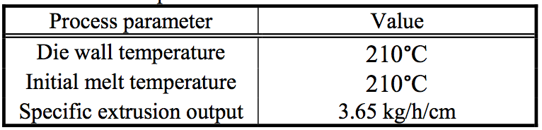
Table 1: Process parameters
Polymer and rheology
The polymer used for this study is a compounded
blend of two grades of ethylene-vinyl acetate copolymer
(EVA):
Where EVA-1 is an EVA manufactured by DuPont which
has a vinyl acetate comonomer content of 18 wt%, a
density of 0.94 g/cm
3
and a melt flow index (MFI) of 0.7 g/10 min (190°C/2.16 kg). EVA-2 is also produced by
DuPont and also has a vinyl acetate comonomer content
of 18 wt%, a density of 0.94 g/cm
3
and a MFI of 2.5 g/10
min (190°C/2.16 kg).
The shear viscosity behavior of this EVA compound
is modeled by the combination of the Cross model[2] for
the shear dependency and the WLF model[3] for the
temperature dependency, according to equations (1) and
(2).
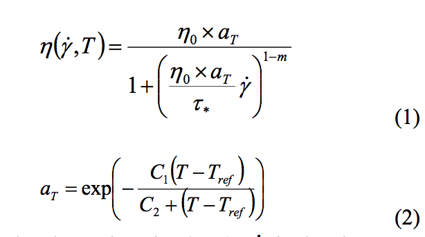
Where ή is the shear viscosity (Pa.s), y is the shear rate
(1/s), T is the temperature (K), ή0 is the zero shear
viscosity (Pa.s), τ* is the characteristic shear stress (Pa)
and m is the pseudo-plastic index. ή0, τ* and m are the
Cross model parameters. The time-temperature
superposition principle (TTS)[4] is included in the Cross
model through the shift factor a
T, which follows a WLF
model, which uses the C
1 and C
2 (K) parameters. The
parameter values used for this work are summarized in
Table 2 and illustrated in Figure 5.
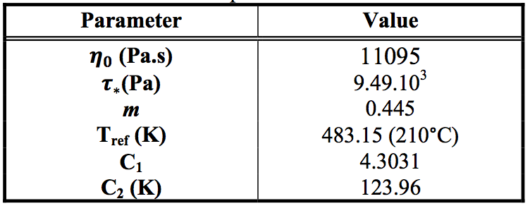
Table 2: Cross and WLF parameters
Finally, the following thermal properties were used: melt
density ρ= 0.795 g.cm
-3, thermal conductivity k=0.25
W.m
-1.K
-1 and specific heat C
p= 3.14 J.g
-1.K
-1.
Flow simulations
The Non-Newtonian, non-isothermal flow
simulation method and governing equations are similar to
those previously published [1].
SolidWorks Flow Simulation 2011 SP1.0[5] was used
to solve the coupled thermal-flow problem and a mesh
with brick elements was built. The boundary conditions
for this model are: (i) a symmetry condition at the
centerline for flow and temperature; (ii) a fully developed
flow at the entrance ; (iii) an initial fluid temperature and a flow rate are imposed at the entrance; (iv) at the outlet
surface (lip opening/exit orifice), the exit pressure is set to
1 atm and; (v) finally, on the flow channel walls, we
assume a non-slip condition (v=0 mm/s) and a uniform
temperature (210°C) is applied.
1 - Full-width die
The die flow channel design was optimized for the
full width configuration, which corresponds to a slot
width of 2050 mm for a total extrusion output of 748.3
kg/h. A flow simulation was run for these conditions with
the geometry illustrated in Figure 3. The calculated
pressure drop is about 15.5 MPa, and Figure 6 shows the
evolution of the melt pressure as a function of the position
along the main flow direction (MD) at the centerline of
the die. Figure 7 shows the velocity contour plot on the
plane defined at mid-plane of the height of the lip land
gap. As can be seen in Figure 8, the exit velocity across
the die width is very uniform.
Because of the relatively high melt viscosity, viscous
dissipation in the die can be a legitimate concern.
However, as shown in Figure 9 the predicted temperature
elevation at die exit due to viscous dissipation is
controlled. The plot shows a maximum temperature of
211.8°C at the mid-plane of the flow stream. By way of
general information, the peak temperature proximate to
the die wall, in the lip land area, was calculated at
214.6°C. As usual for non-isothermal flow assuming a
uniform die wall temperature, the warmer portion of the
melt is observed near the die ends of the die width.
Finally, another critical parameter in this study is the
residence time distribution in the die. For this study, the
numerical estimation of the residence time is very
challenging due to the existence of low flow rate regions.
The best method in this case is to perform a virtual
injection of particles in the flow. Residence time is
evaluated by tracking the particles from the entrance to
the exit. This numerical method is relatively common and
many publications can be found for RTD and mixing
performance estimation in twin screw extrusion[6 -
8]. This method provides a relative comparison of residence time
distribution for different die configurations. There are
many parameters that define a particle injection study, like
for example the type of particle material, the particle size,
the initial temperature etc… These parameters will not be
detailed here, however, in order to compare the die deckle
variations, these parameters are kept constant throughout
the study. One thousand particles were injected in a plane
near the entrance of the manifold channel. On each
resulting particle trajectory, the trajectory time is plotted.
The resulting plot is shown in Figure 10. This particle
injection study yields to statistics of major interest, like
for example, the cumulative residence time distribution curve shown in Figure 11, and the residence time
envelope, shown in Figure 12.
2 - Externally deckled die
Two flow simulations were carried out for the
situation where external deckles are used, corresponding
to deckles of 250 mm per side (total slot width of 1550
mm) - see Figure 13 - and deckles of 500 mm per side
(total slot width of 1050 mm) – see Figure 14.
The total extrusion output was adjusted with the slot
width to keep the specific extrusion output constant, at
3.65 kg/hr/cm. Consequently, the calculated melt pressure
drop in the die for both deckle configurations is close to
that of the full die width. Specifically, the 250 mm deckle
configuration resulted in a melt pressure drop through the
die of 14.7 MPa and the 500 mm deckle configuration in a
melt pressure drop through the die of 14.6 MPa. For
illustrative purposes, the melt pressure contour plot
through the die flow channel using the 500 mm deckles is
shown in Figure 15.
Velocity contour plots for the externally deckled die
are shown in Figure 16 and Figure 17 for the 250 mm
deckles and the 500 mm deckles respectively. These plots
show the occurrence of a large area upstream the deckles
where the flow velocities are low. These zones can be
considered stagnation areas. In order to understand the
flow patterns better, velocity vectors are plotted on top of
the contour plots in the deckle area, near the exit. In
particular, Figure 18 shows the existence of a strong
velocity gradient in the area of the slot proximate to the
deckle extremity. This gradient is caused by the excess
polymer flowing from a portion of the area upstream and
behind the deckle. This phenomenon is further
characterized by the exit velocity profiles shown in Figure
19.
The thermal characteristics of the flow in the
externally deckled dies are illustrated by the temperature
contour plot shown in Figure 20. This shows a classic
shear heating effect on the side walls of the entrance
channel, along the back wall of the manifold channel.
However, the melt is dissipating heat in the area upstream
and behind the deckled region to match the die wall
temperature owing to the very low flow velocities. As a
result, this cold area provides a good correlation to the
stagnant melt flow regimes.
Capturing the residence time distribution in the
deckled configuration proved challenging; and two steps
are necessary to really evaluate the whole die flow
pattern. When using the particle injection near the
manifold channel entrance similarly to what is done for
the full width die, it is possible to compare the residence
time figures to that of the full width reference. However, this particle injection method does not fully capture the
high residence time area at the very ends of the flow
channel and immediately upstream the deckles, as shown
by the particle trajectories in Figure 21 and Figure 22.
These trajectories however may be seen as the measurable
majority of the flow reaching the die exit and therefore, it
is interesting to study their statistics compared to the full
width configuration. For example the cloud plots of
trajectory time versus trajectory flow length for all three
configurations (Figure 23) show interesting results. The
larger the deckles, the longer the residence time, despite
the shorter flow lengths associated with the active width
of the die. Interestingly, the maximum flow length for the
250 mm deckle configuration is very close to that of the
full width configuration because of the flow trajectories
inside the low velocity region ultimately exit the die near
the deckle inner end defining the exit slot. The RTD
curves (Figure 24) characterize residence time associated
with external deckles.
Nevertheless, these figures are not complete because
as mentioned before, the trajectories do not capture the
regions near the end of the manifold channel. It is possible
to obtain a representation of the residence time in these
regions when injecting particles along the back of
manifold channel, as close as the entrance as possible.
Figure 25 shows that the residence time in these regions
can be well in excess of 300 s for the 250 mm external
deckle configuration, while Figure 26 illustrates a
residence time greater than 1,500 s for the 500 mm deckle
configuration. While these numbers should not be
interpreted as absolute values, they provide a good
indication of the flow pattern and RTD in the externally
deckled dies. As can be appreciated from this modeling,
residence time increases exponentially with external
deckle width.
3 - Internally deckled die
Similar to the flow simulations for the external deckle
system, two flow simulations were run for the internal
deckle scenarios with 250 mm and 500 mm deckles
respectively. The principles applied for the boundary
conditions for the internal deckle models were the same as
for the external deckle flow simulations.
Calculated pressure drop is about 14.8 MPa for both
conditions, which is comparable to the full width model.
This is expected because the specific output is kept
constant relative to the effective slot width for all the
simulations. For illustration purposes, the pressure
contour plot for the 500 mm internal deckle scenario is
shown in Figure 27.
Velocity contour and vector plots are shown in Figure
28 and Figure 29 respectively, for the 250 mm internal
deckles; and in Figures 30, 31 respectively, for the 500 mm internal deckles. The internal deckle configuration
results in higher overall flow velocities compared to the
corresponding external deckle widths. The internal deckle
device beneficially replaces this low velocity regimes
present in the flow channel when using the external
deckles. Also, the flow velocities at the die exit are much
improved. Compared to the external deckle scenario,
internal deckles result in a much more uniform velocity
profile at the exit of the die, particularly at the end regions
of the deckled die width. The velocity surge that was
present with external deckles at the die exit near the
deckle is nonexistent with internal deckles. Figure 32
shows the flow profile at the die lips. It exhibits slightly
more end flow when wider deckles are used. The die
preland, which is designed to uniformly distribute the
flow across the full slot width, becomes less adapted for
narrower slot widths. However, this behavior is acceptable
because even when using 500 mm deckles, the flow
distribution is satisfactory and well within the range of
correction from typical lip adjustment systems.
The melt temperature pattern is very similar to that of
the full width die, with temperature gradients from the
wall to the mid-plane of the channel. The temperature
contour for the 250 mm internal deckle configuration is
shown in Figure 33. The temperature profile at the die lips
exhibits slightly warmer melt near the ends, which is a
signature of shear heating in the flow channel. The
intensity of this phenomenon however is largely
insignificant as demonstrated by the modest temperature
increase (1.8°C).
The virtual particle injection method was used to
evaluate the RTD for internal deckle configurations. The
resulting particle tracings are shown in Figure 34 and
Figure 35 when injecting particles near the entrance of the
manifold channel for the 250 mm internal deckle
configuration and the 500 mm internal deckle
configuration respectively. This analysis shows a
relatively streamlined flow pattern, equivalent to that of
the full width die in both cases. The relationship between
residence time and flow length is shown in cloud graph in
Figure 36. The shapes of the RTD clouds show that
internal deckle configurations behave very similarly to a full width die. Correspondingly, the shapes of the RTD
curves (shown in Figure 37) exhibit a behavior of
similarity between internally deckled and the full width
configuration dies. The main different lays in the smaller
values of maximum residence time when using wider
deckles (narrower slot width). Finally, a direct comparison
of RTD curves between the internal style and external
style deckles is shown in Figure 38 for the 250 mm deckle
configurations and Figure 39 for the 500 mm deckle
configurations.
Conclusion
CFD was successfully used to compare two
styles of deckle systems commonly used in flat film or
sheet extrusion. The use of advanced CFD tools like
virtual particle tracking allows for the performance
evaluation of the polymer flow between two different
deckle configurations. For instance, it is possible to
illustrate and quantify the flow stagnation upstream of
external deckles. Flow non-uniformity with this system is
also demonstrated. By comparison, it was found that
internal deckle systems compare very similarly to full
width dies as the flow at the exit of the die remains fairly
uniform and unaffected by the die width.
[1] O. Catherine, SPE-ANTEC Tech Papers (2011)
[2] M. M. Cross, Polymer Systems: Deformation and
Flow (1968)
[3] M. L. Williams, R. F. Landel and J. D. Ferry, J. Am.
Chem. Soc., 77, 3701 (1955)
[4] J. D. Ferry, Viscoelastic properties of polymers. 3rd
edit. (1980)
[5] Dassault Systèmes, S.A.
[6] V. L. Bravo, A. N. Hrymak, and J. D. Wright, Polym.
Eng. Sci., 44: 779–793 . (2004)
[7] X. –M Zhang, L.-F Feng, W.-X Chen and G.-H Hu,
Polym. Eng. Sci., 49: 1772–1783 (2009)
[8] F. Ilinca, J. F. Hetu, Intern. Polym. Proc., XXV 4:
275-285 (2010)
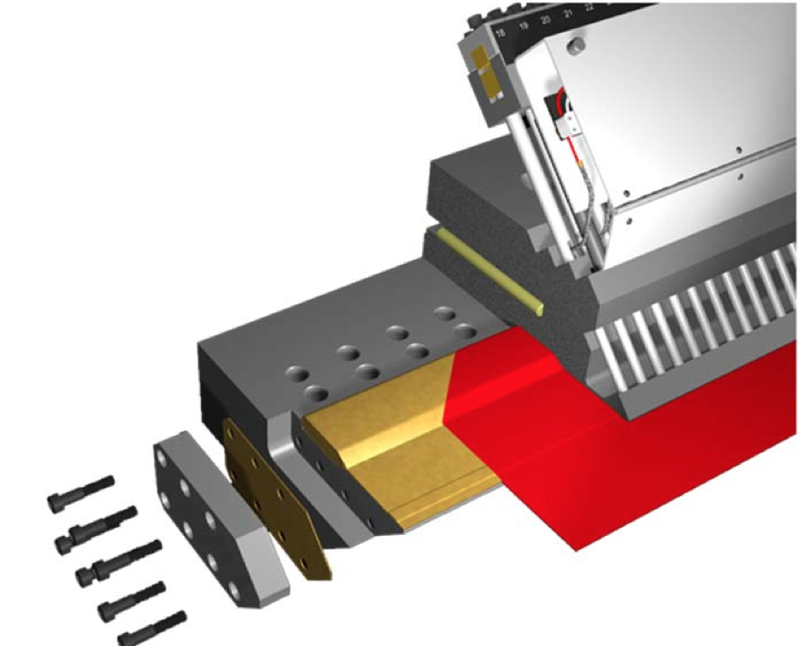
Figure 1. Schematic of a fixed width internal deckle system
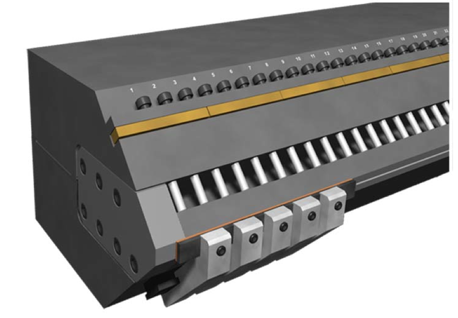
Figure 2: External deckle system consisting of (1) a seal, (2) the deckle seal plate and (3) retaining fingers with (3) set screws
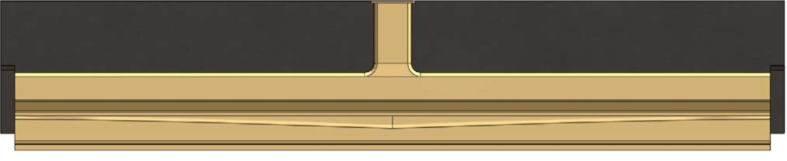
Figure 3: Die geometry used for the flow studies – plane view
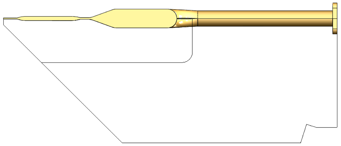
Figure 4: Die geometry used the flow studies – side view
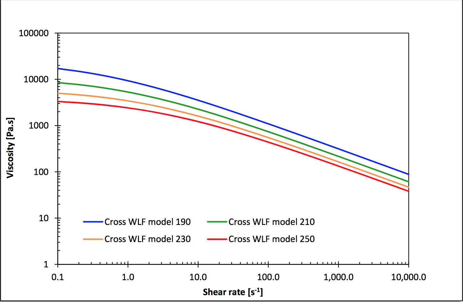
Figure 5: Viscosity curves of the selected Cross WLF model
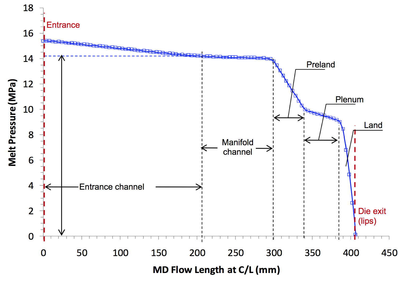
Figure 6: Pressure drop profile at the centerline in the main flow direction (machine direction), from entrance (0 mm) to exit (400 mm), showing the contribution of the flow channel portions
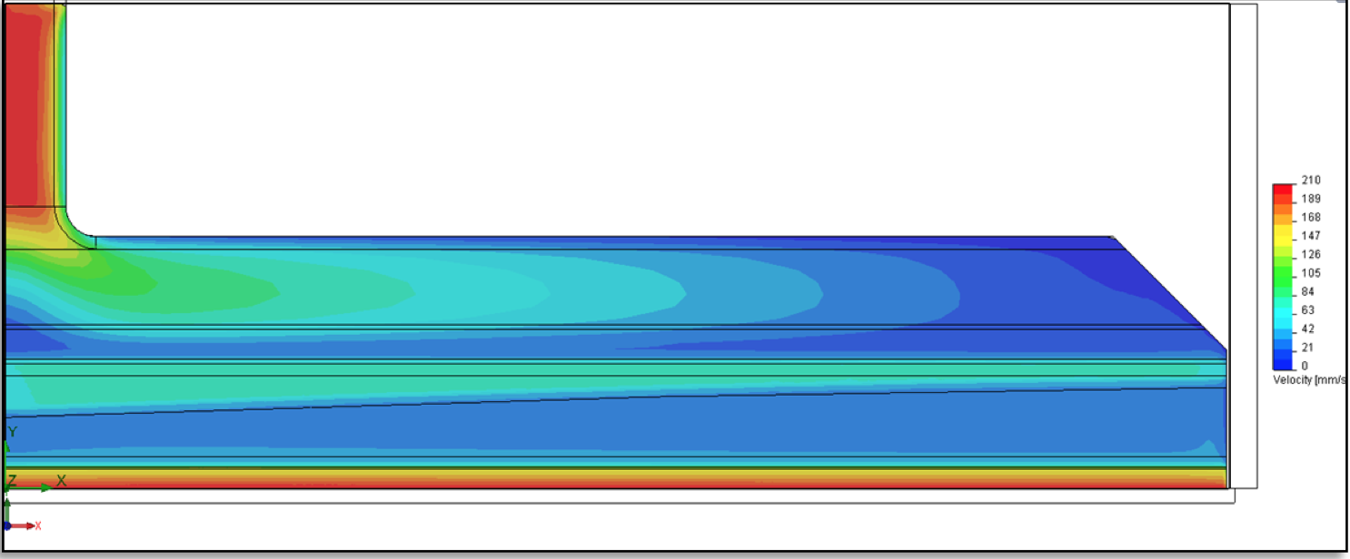
Figure 7: Velocity contour plot on the plane defined a mid-height of the lip land
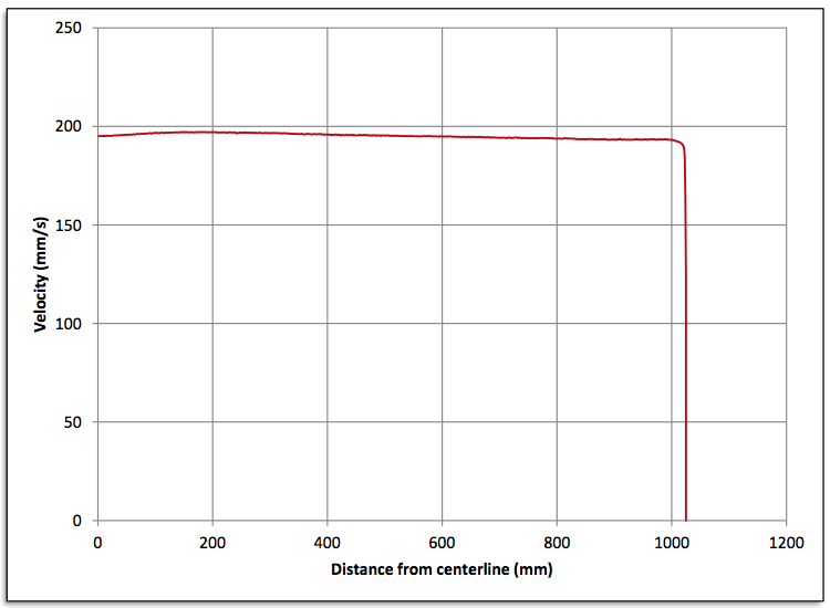
Figure 8: Computed exit velocity profile
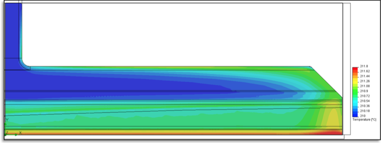
Figure 9: Temperature contour plot on the plan defined at mid-height of the lip land gap
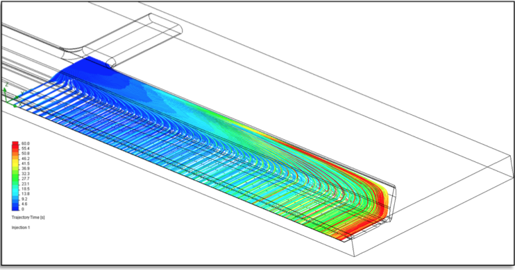
Figure 10: Estimation of residence time distribution by virtual particle injection
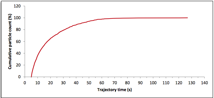
Figure 11: RTD (Residence Time Distribution) curve for full width die
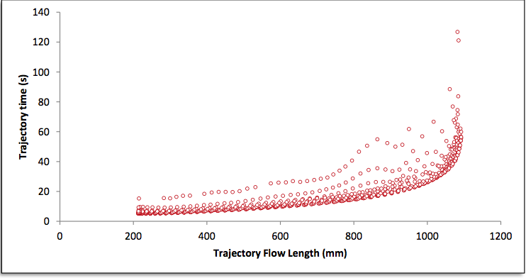
Figure 12: Trajectory time across the die width as a function of trajectory length for full width configuration
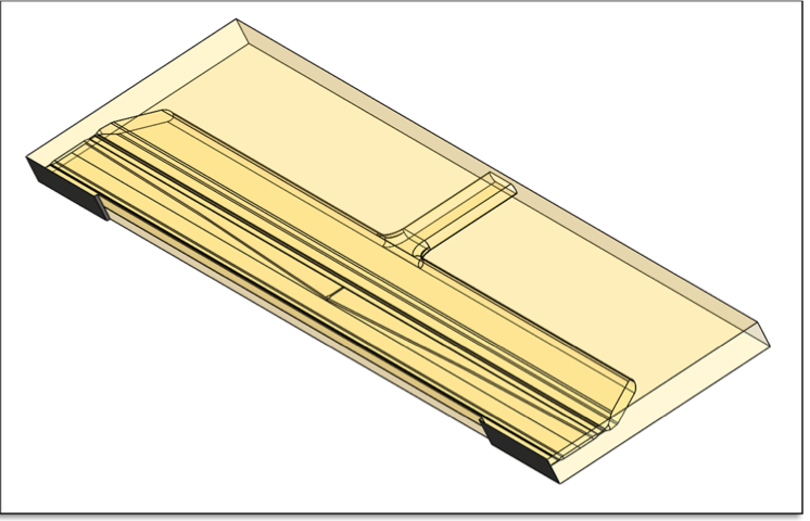
Figure 13: Die geometry for 250 mm external deckles
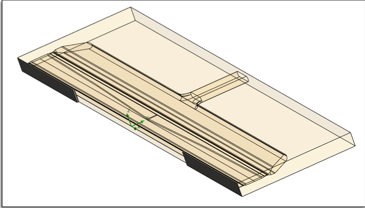
Figure 14: Die geometry for 500 mm external deckles
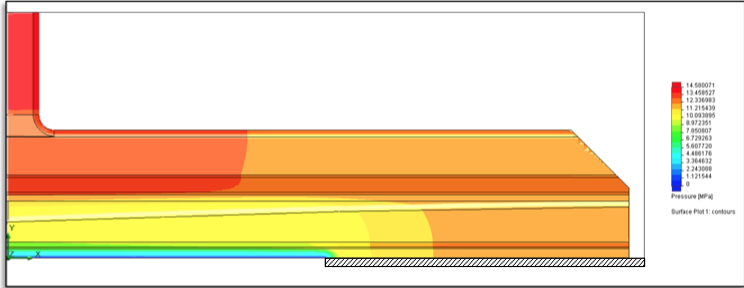
Figure 15: Melt pressure distribution map in the die using the 500 mm external deckles
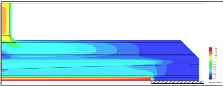
Figure 16: Velocity contour plot through the flow channel with 250 mm external deckle
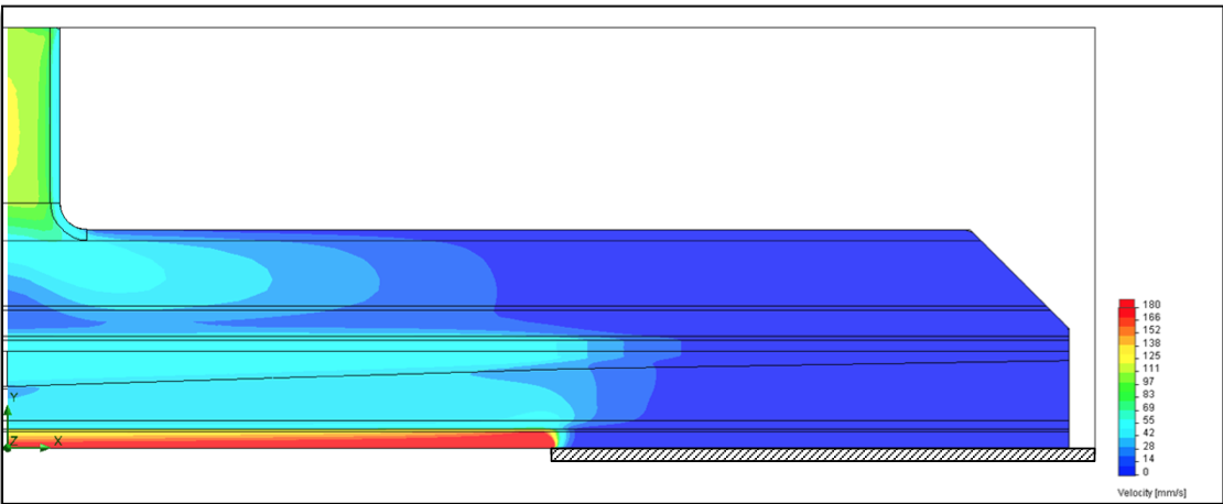
Figure 17: Velocity contour plot through the flow channel with 500 mm external deckles
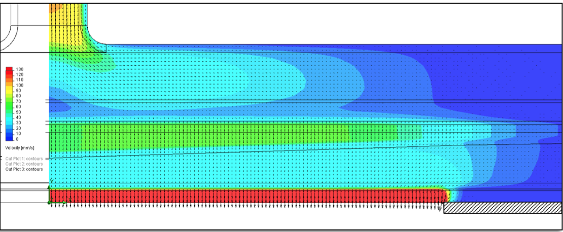
Figure 18: Velocity contour plot superimposed with velocity vectors representing the direction and the intensity of the velocity field

Figure 19: Exit velocity profiles for the externally deckled die
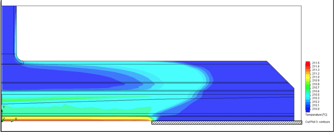
Figure 20: Temperature contour plot on midplane for the 500 mm external deckle configuration
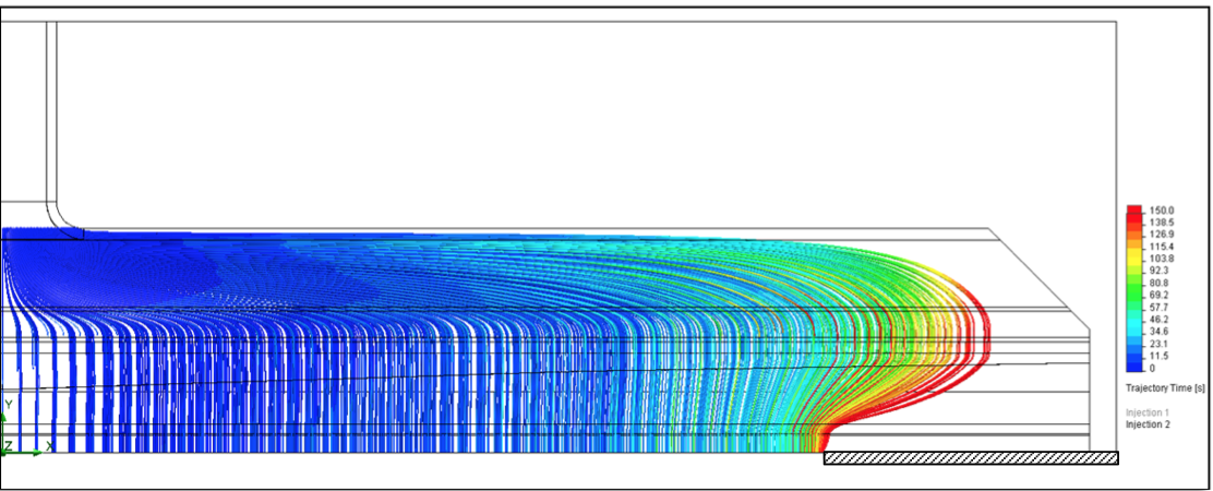
Figure 21: Result of virtual particle injection for the die with the 250 mm external deckle configuration - Particles injected near the entrance to the manifold channel
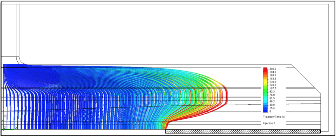
Figure 22: Result of virtual particle injection for the die with the 500 mm external deckle configuration - Particles injected near the entrance to the manifold channel
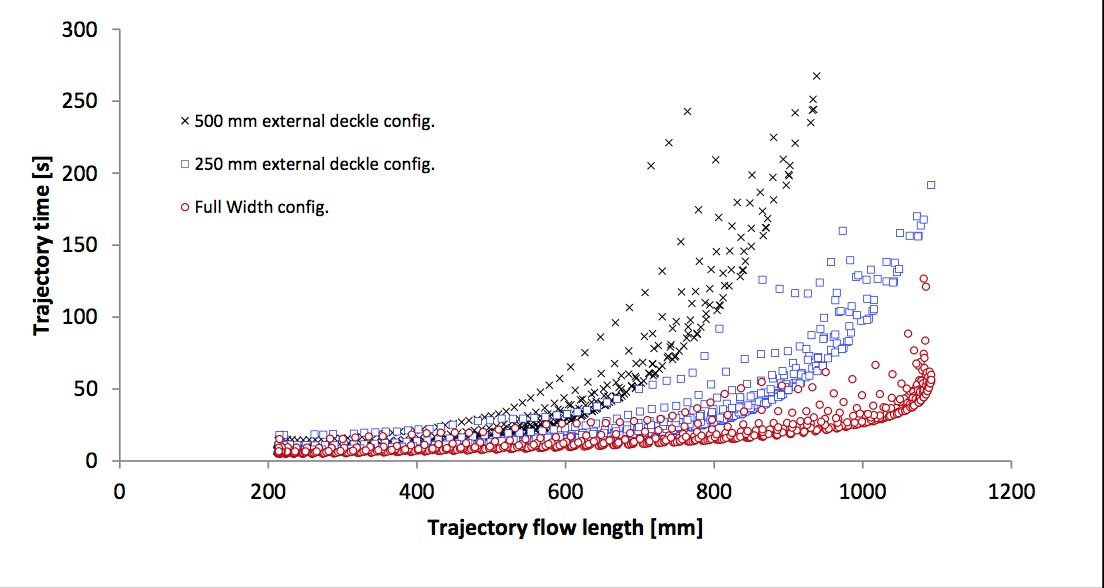
Figure 23: Comparison of trajectory time to trajectory flow length clouds for external deckle configurations
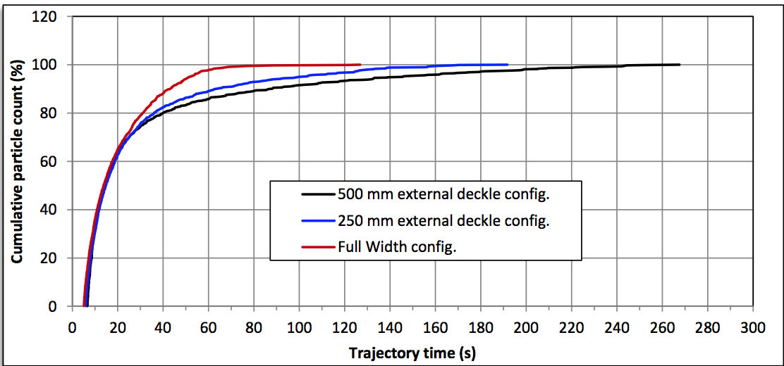
Figure 24: Comparison of cumulative residence time distribution curves for external deckle configurations
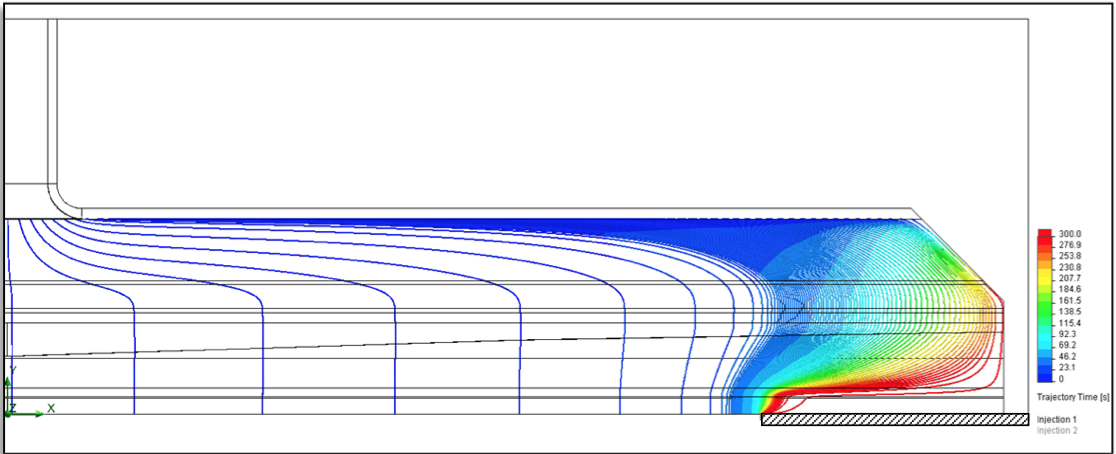
Figure 25: Result of virtual particle injection for the die with the 250 mm external deckle configuration - Particles injected at the midplane near the back wall of the manifold channel
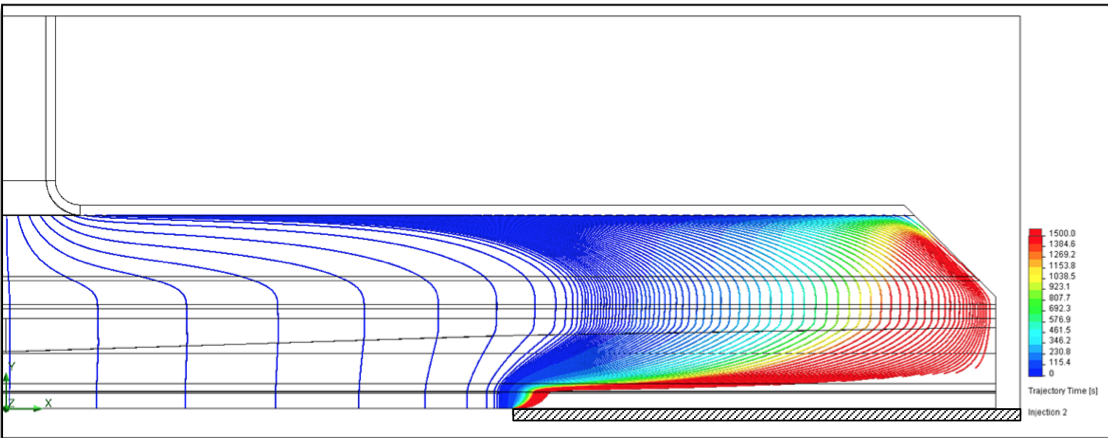
Figure 26: Result of virtual particle injection for the die with the 500 mm external deckle configuration - Particles injected at the midplane near the back wall of the manifold channel
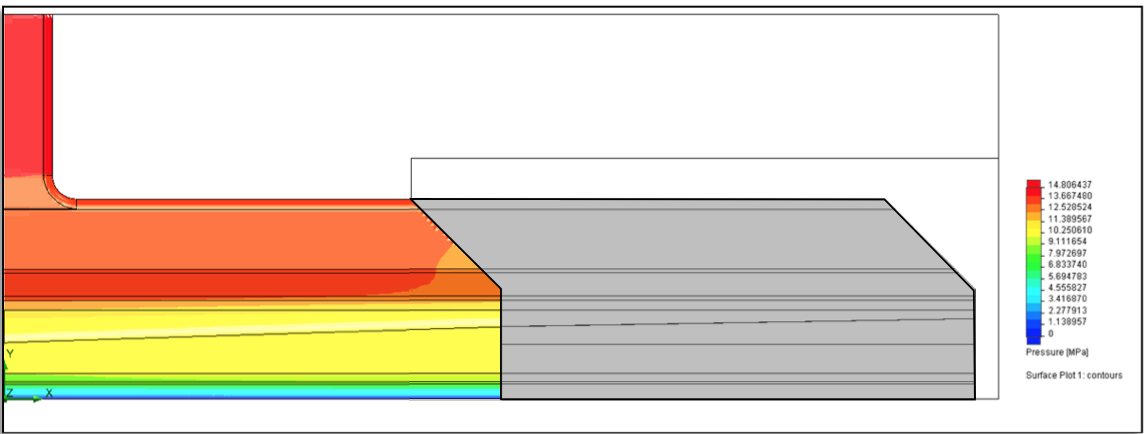
Figure 27: Melt pressure contour plot for the 500 mm internal deckle configuration
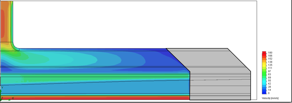
Figure 28: Velocity contour plot for the 250 mm internal deckle configuration
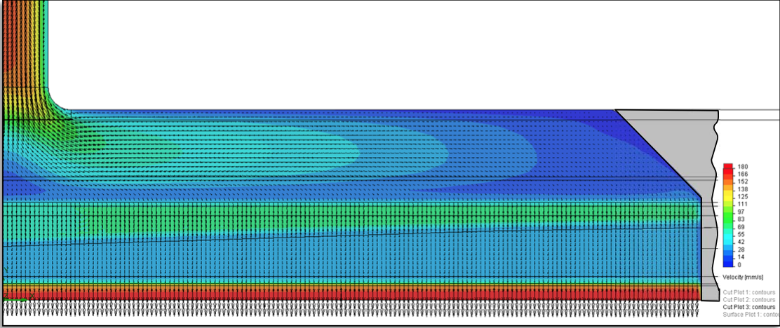
Figure 29: Velocity contour plot superimposed with velocity vectors representing the direction and the intensity of the velocity field for the 250 mm internal deckle configuration
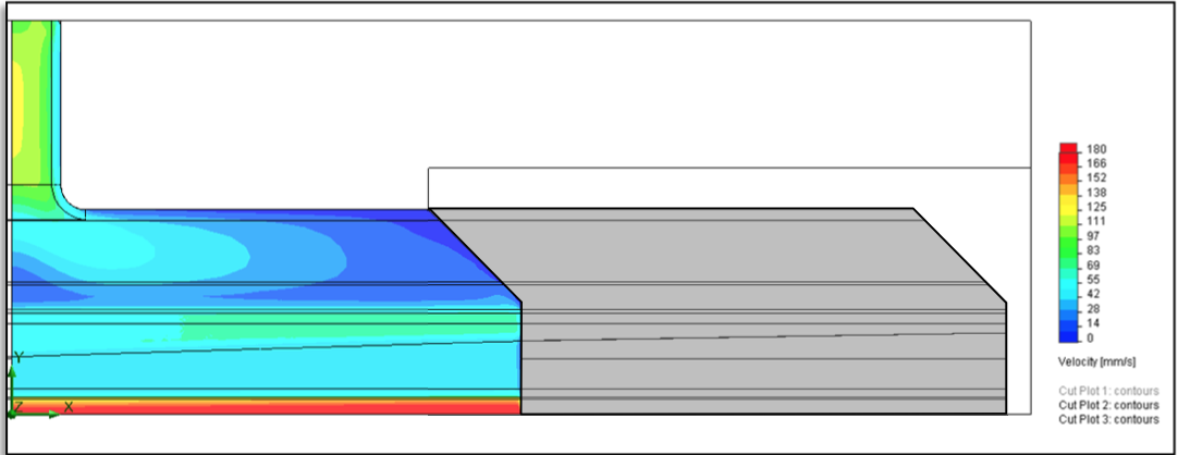
Figure 30: Velocity contour plot for the 500mm internal deckle configuration
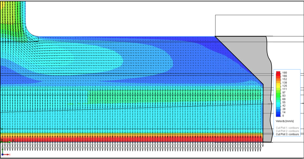
Figure 31: Velocity contour plot superimposed with velocity vectors representing the direction and the intensity of the velocity field for the 250 mm internal deckle configuration
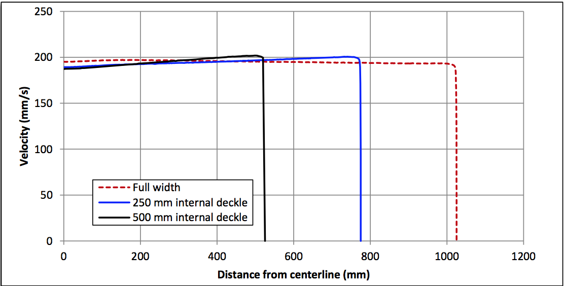
Figure 32: Velocity profile at the die lips (at mid plane)
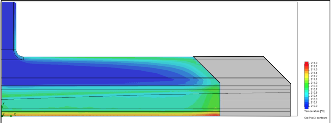
Figure 33: Melt temperature contour plot on the mid plane of the die for the 250 mm internal deckle configuration
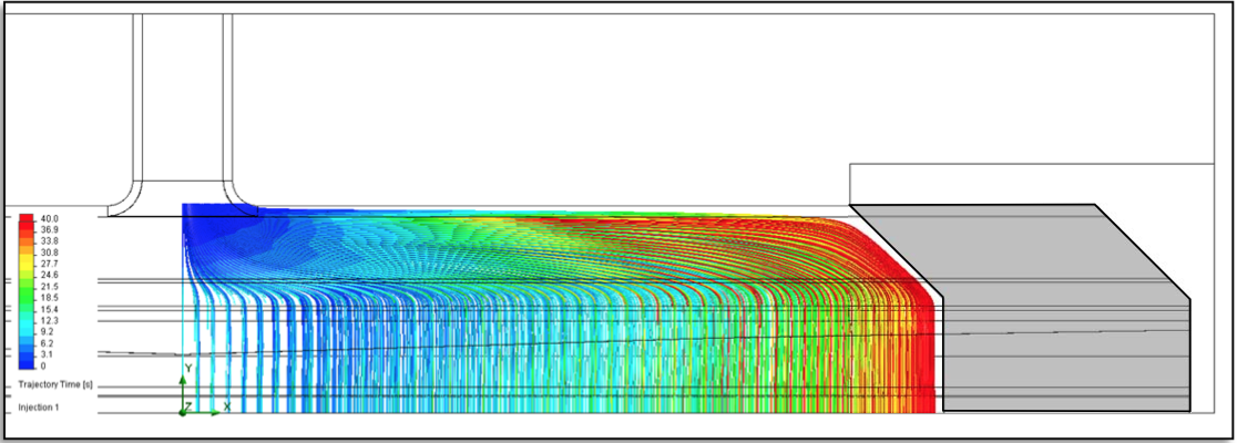
Figure 34: Result of virtual particle injection for the die with the 250 mm internal deckle configuration - Particles injected at the midplane near the entrance of the manifold channel
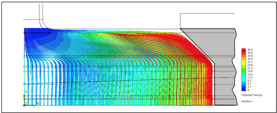
Figure 35: Result of virtual particle injection for the die with the500 mm internal deckle configuration - Particles injected at the midplane near the entrance of the manifold channel
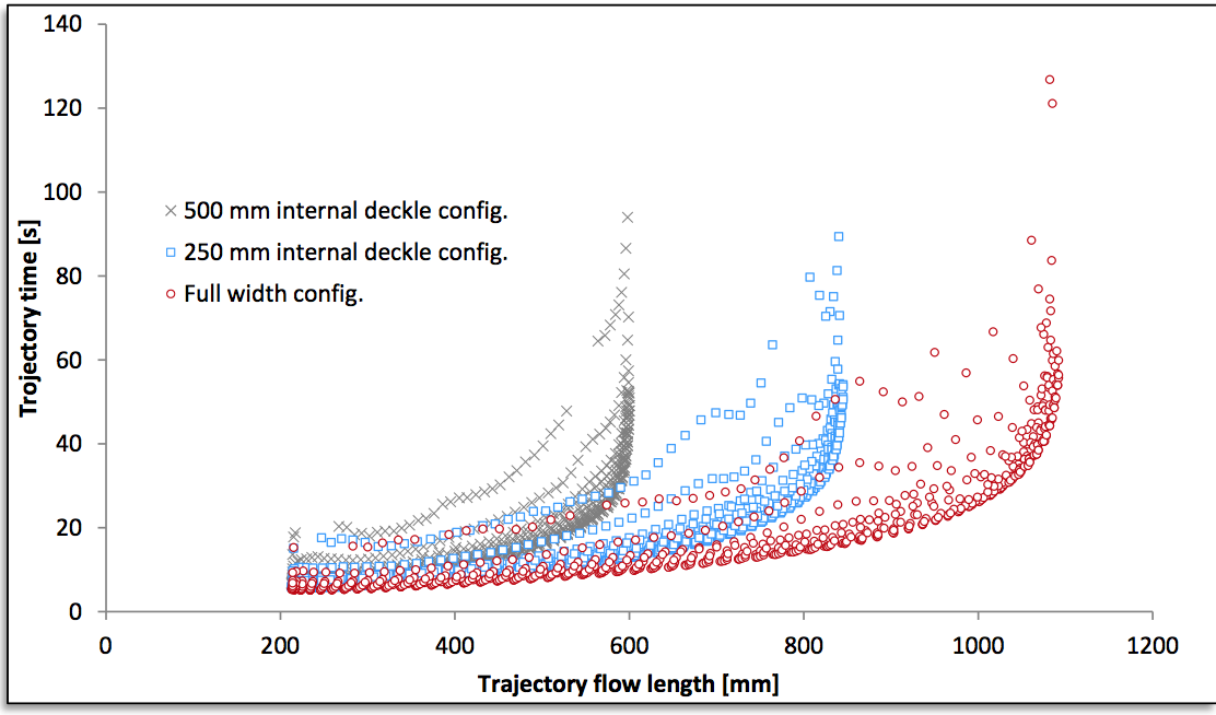
Figure 36: Comparison of trajectory time to trajectory flow length clouds for internal deckle configurations
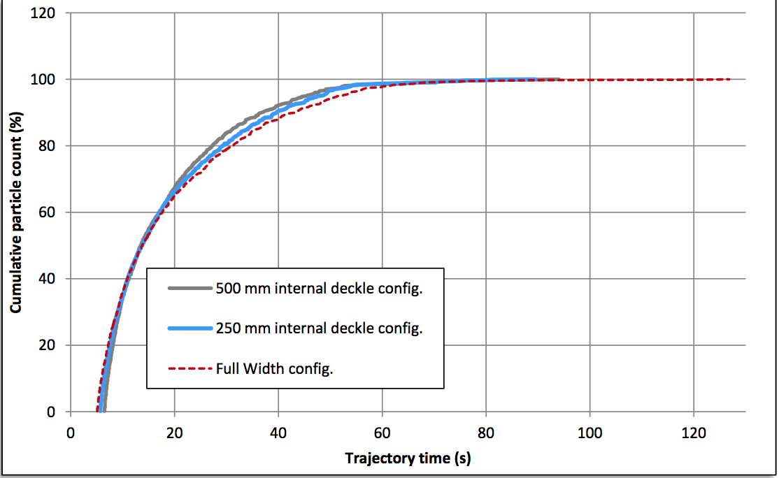
Figure 37: Comparison of cumulative residence time distribution curves for internal deckle configurations
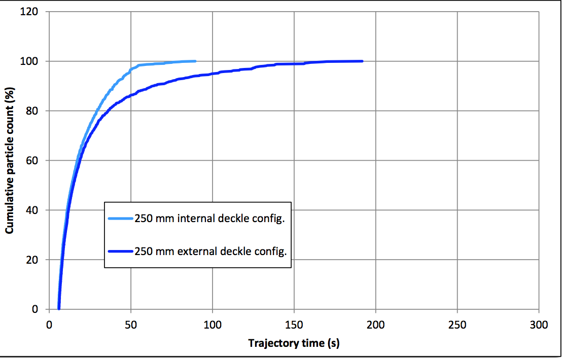
Figure 38: Comparison of RTD curves for internal and external deckles (250 mm)
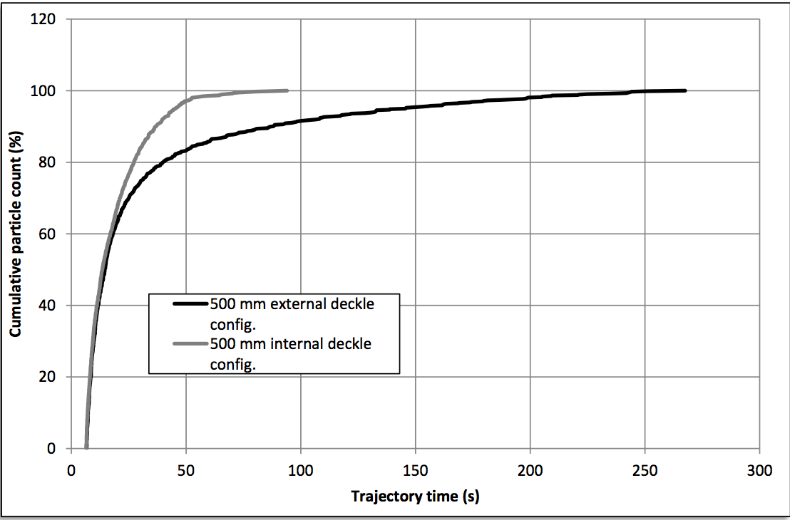
Figure 39: Comparison of RTD curves for internal and external deckles (500 mm)
Return to
Paper of the Month.